Visualising Parallelisation

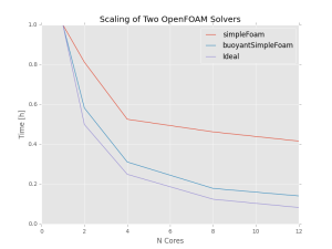
Today’s post is based on something I see all too often.  In CFD, to make a simulation run faster, we typically use more cores and to analyse how much faster it is per processor core we add, we record the time.  This is great as it gives the time taken, which in most cases is lower when you use more cores.  Then, because we are visual beings and numbers in tables don’t give us as much insight as a graph, we plot the data:

Time against number of cores for two OpenFOAM solvers.

What a beautiful plot (if I say so myself), but what does it really tell us?  It shows:

• Both A and B get quicker with more cores.
• A is faster than B.
• A does not scale as fast as an ideal scaling.

This is the graph I often see, and it frustrates me because there is more that you can do with the data that tells us a bit more about how the solver/problem scales.  Let me introduce here two concepts, the first is speed up and the second is parallel efficiency; each can be derived from the data above and both tell us something more.

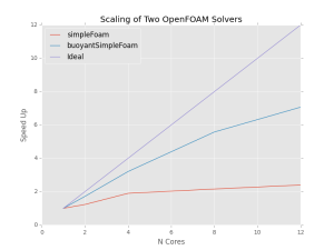
Speed up is the (inverse) ratio of the time taken for the parallel run to the time taken for a run on a single core.  Thus with a perfectly linear scaling, the speed up is equal to the number of cores and unless the code is super fantastic, it will fall somewhere below this line:

Speed up against number of cores for two OpenFOAM solvers.

This tells us how the solver and problem scale, not just how long it took; whether it is linear, reaching a plateau or barely faster than a single core simulation.  We do lose some information about the absolute time taken, but this can be regained by using the absolute speed up instead, which uses the fastest serial time to solve the problem (rather than the time for the same code on a single core).

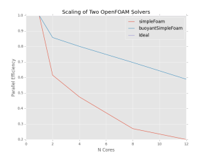
The other metric which is potentially useful is parallel efficiency, which is the speed up divided by number of cores.  This tells us how close we are to linear speed up, with a value of 1 equalling perfect scaling.  The graph below shows that for the OpenFOAM solvers tested (for the specific problems), the returns on using more cores are diminishing (rapidly in the case of simpleFoam).

Parallel efficiency against number of cores for two OpenFOAM solvers.

Arguably, this metric is of limited use when it comes to absolute performance, however it is highly insightful when analysing throughput for a limited resource.  For example, if you had to run both simulations in the above figure, instead of using 12 cores for simpleFoam and buoyantSimpleFoam sequentially, we could use 4 for simpleFoam and 8 for buoyantSimpleFoam to get both answers quicker.

Neither of these metrics is a new thing in high performance computing, but CFD is all too easily (and too often) scaled without much thought behind the benefits (or not) of doing so.  Unfortunately, much like the cursed pie chart, I expect I have not seen the last plot of time against cores to “show scaling”, but at least I have shown here that other y axes exist.

Thermal Convection Simulation in OpenFOAM

As you may have guessed from the title, this post is a technical one, so if you have no interest in OpenFOAM, feel free to skip.

Part of my current work involves simulating forced and free convection using OpenFOAM which is a CFD package that simultaneously blesses and curses you with freedom.  In more recent versions, anyone using a steady state solver without setting their divergence schemes with a bounded keyword would have incurred the solvers wrath and been issued with iteration after iteration of complaint.  This is all very fine, but I am using a bounded divergence scheme (Self-Filtered Central Differencing) and unsteady in time, so I don’t need to set the bounded keyword, right?  Well, that is what I thought, until I tried to work out why I was getting temperatures in the order of -200C in just a few cells (N.B. the working ‘fluid’ would be solid at this temperature!).  No amount of under-hood tinkering managed to fix these numerical gremlins until I found the answer: the bounded keyword.  With the inclusion of the following line all my problems went away:

div(phi,T) bounded Gauss <interpolationScheme>;

So it seems that, even if the solver doesn’t complain, a bounded keyword may be necessary to get your simulation to behave itself.  This has left me with a few questions, which I will hopefully find answers to in due course:

• Does including the correction ever incur a penalty other than time?
• Why not include the boundedness correction for all convective terms by default?